Calculating spatial metrics for IUCN RLE assessments

Aniko Toth, José R. Ferrer-Paris, Calvin K.F. Lee, Nicholas J. Murray

2026-01-27

1. Introduction

In this vignette, we provide an example of using the tools within redlistr to assess the spatial criteria of the IUCN Red List of Ecosystems. These criteria assess the change in the extent of an ecosystem over time (Criterion A) and properties of the geographic distribution size (Criterion B). Both of these criteria require the use of maps of ecosystem distributions.

We begin by loading the packages we need for data import and for calculation of the spatial metrics. Please ensure that these are already installed.

library(terra)
library(redlistr)

2. Importing data

We first import the spatial data we want to analyse. In this vignette, we will be using two example distributions included with the package. They are mangrove distributions from the northern regions of Western Port Bay, Victoria, Australia. The first distribution is from Giri et al., (2011), and represents mangrove distribution in 2000. The second distribution is a classification map generated using the XGBoost package and data from Landsat 8, and represents mangrove distribution in 2017. Both of these geographic distributions are stored as rasters, and a raster value of 1 denotes presence.

We use function rast from the terra package to read these rasters. This function requires a valid path to find the files with the raster data. In this case both files are included in the redlistr package, so we use the system.file function to find the path to those files. More information about formats and functions of the terra package can be found here.

mangrove.2000 <- rast(system.file("extdata", "example_distribution_2000.tif", 
                                    package = "redlistr"))
mangrove.2017 <- rast(system.file("extdata", "example_distribution_2017.tif", 
                                    package = "redlistr"))

Alternative formats

See vignette Ecosystem distribution data in raster and vector format for instruction on how to read ecosystem distribution data in other formats.

Plotting out data

We plot the data to view the two mangrove distributions to get a general idea of how the distribution might have changed over time.

plot(mangrove.2000, col = "grey30", legend = FALSE, main = "Mangrove Distribution")
plot(mangrove.2017, add = T, col = "darkorange", legend = FALSE)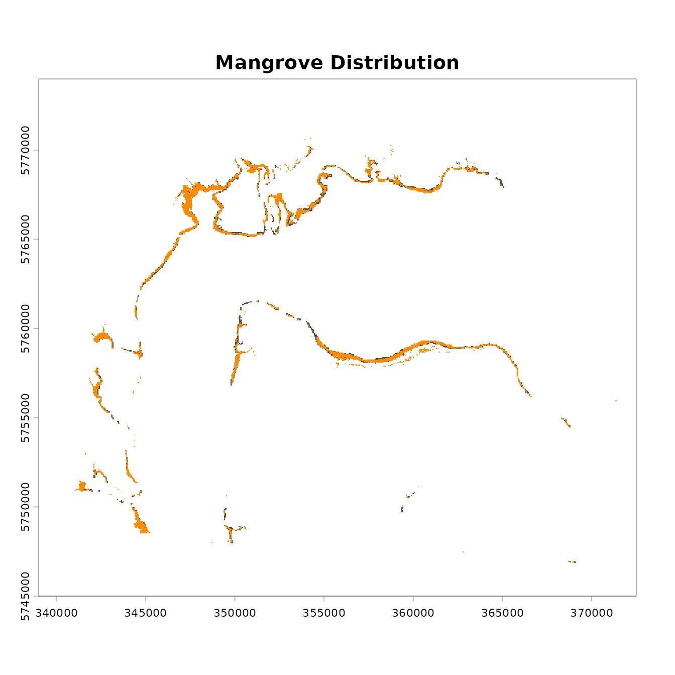

We can see that there has been some change in mangrove cover, although the losses appear to be relatively minor.

At this stage it is important to check that the data are georectified (in the right location on Earth). This can be achieved by simply plotting the map and checking the coordinates. Otherwise, check the distribution maps against satellite images, perhaps by using packages such as ggmap, plotgooglemaps, googleVis etc. It is also important to check that the data are suitable for the task at hand.

3. Basic information for the data

We now use some of features of redlistr to get some basic information on the ecosystem distribution. However, before proceeding, we check their resolution (grain size), extent, and spatial properties. Specifically, the coordinate reference system (CRS) of the datasets must be measured in metres, and must be consistent between layers you wish to compare.

is.lonlat(mangrove.2000) 

## [1] FALSE

is.lonlat(mangrove.2017)

## [1] FALSE

# If TRUE, they must be transformed to a projected coordinate system

crs(mangrove.2000) == crs(mangrove.2017)

## [1] TRUE

Reprojection can be done by using the terra::project function. Be sure to choose a coordinate reference system that is appropriate to your study system.

We start by calculating the area of the ecosystem. Area is calculated here using the pixel count method, where the number of pixels classified as the ecosystem of interest is multiplied by the area of each pixel, giving the area of the ecosystem distribution. The area calculated is provided in square kilometres.

a.2000 <- getArea(mangrove.2000)
a.2000

##                       layer value     area
## 1 example_distribution_2000     1 13.65908

a.2017 <- getArea(mangrove.2017)
a.2017

##                       layer value     area
## 1 example_distribution_2017     1 12.33667

The results: at time 1 (2000), the ecosystem was 13.6590844 km2, and at time 2, (2017) the ecosystem was 12.3366736 km2.

Rasters with multiple ecosystems or layers

The getArea function is capable of processing rasters with multiple ecosystems and layers. For example you can also calculate areas for both layers at once by combining them into a raster stack:

a <- getArea(c(mangrove.2000, mangrove.2017))

See vignette Scaling up Red List of Ecosystem assessments for instruction on how to work with multiple ecosystem maps.

4. Assessing Criterion A

The IUCN Red List of Ecosystems criterion A requires estimates of the magnitude of change over time. This is typically calculated over a 50 year time period (past, present or future) or against a historical baseline (IUCN 2024). The first step towards achieving this change estimate over a fixed time frame is to assess the amount of change observed in your data.

Area change

Area change can be calculated for one of two scenarios: multiple ecosystems over two time slices using getAreaChange(), or one or more ecosystems over multiple time slices using getAreaTrend().

The getAreaChange function takes two inputs in the same format. It calculates the difference in area between two datasets, which can contain multiple ecosystems. It can accept data from data.frame such as those output by the getArea() function, SpatRaster, SpatVector or sf objects with POLYGON geometries. Make sure to provide area measure in $km^2$ if you are using a data.frame as the input. Note that when providing data frame and polygon inputs, the column name with unique ecosystem labels must be included in the function call. If the column name is different in the two inputs, both names must be provided in the same order as the input datasets.

# input rasters
area.change <- getAreaChange(mangrove.2000, mangrove.2017)

# input data frames 
# value is the column that identifies the ecosystem in both tables.

area.change <- getAreaChange(a.2000, a.2017, value) 

The getAreaTrend can be used to work with multiple maps representing different ecosystem types and time frames. See vignette Scaling up Red List of Ecosystem assessments for instruction on how to work with multiple ecosystem maps.

Rate of change

In the Red List of Ecosystems, two methods are suggested to determine the rate of decline of an ecosystem, each of which assumes a different functional form of the decline (IUCN 2024). The proportional rate of decline (PRD) is a fraction of the previous year’s remaining area, while the absolute rate of decline (ARD) is a constant fraction of the area of the ecosystem at the beginning of the decline (IUCN 2024). These rates of decline allow the use of two or more data points to extrapolate to the full 50 year timeframe required in an assessment.

The annual rate of change (ARC) uses a compound interest law to determine the instantaneous rate of change (Puyravaud 2003).

To estimate the rate of changing using these methods, we use the getDeclineStats function.

decline.stats <- getDeclineStats(a.2000$area, a.2017$area, 2000, 2017, 
                                 methods = c('ARD', 'PRD', 'ARC'))
decline.stats

##   absolute.loss        ARD       PRD        ARC
## 1      1.322411 0.07778887 0.5972003 -0.5989906

Each method represent a different shape of decline. For further information about the choice of each of these methods to extrapolate refer to the IUCN Red List of Ecosystems guidelines (IUCN 2024).

Now, it is possible to extrapolate, using only two estimates of an ecosystems’ area, to the full 50 year period required for a Red List of Ecosystems assessment.

extrapolated.area <- futureAreaEstimate(a.2000$area, year.t1 = 2000, 
                                        ARD = decline.stats$ARD, 
                                        PRD = decline.stats$PRD, 
                                        ARC = decline.stats$ARC, 
                                        nYears = 50)

## Warning in futureAreaEstimate(a.2000$area, year.t1 = 2000, ARD = decline.stats$ARD, : 'futureAreaEstimate' is deprecated.
## Use 'extrapolateEstimate' instead.
## See help("Deprecated") and help("redlistr-deprecated").

extrapolated.area

##   forecast.year A.ARD.t3 A.PRD.t3 A.ARC.t3
## 1          2050 9.769641 10.12401 10.12401

50 years from our first estimate is the year 2050.

As we included all three methods of calculating rate of decline currently included in the package, the results produced shows three estimated areas under the various decline scenarios. It is important to note that this relatively simple exercise is founded on assumptions that should be fully understood before submitting your ecosystem assessment to the IUCN Red List of Ecosystems Committee for Scientific Standards. Furthermore, the guidelines suggest using area estimates from more than two time points to estimate change, and providing a measure of uncertainty if possible. Please see the guidelines (IUCN 2024) for more information.

If we were to use the Proportional Rate of Decline (PRD) for our example assessment, our results here will be suitable for criterion A2b (Any 50 year period), and the percent loss of area is:

predicted.percent.loss <- (extrapolated.area$A.PRD.t3 - a.2000$area)/a.2000$area * 100
predicted.percent.loss

## [1] -25.88078

4. Assessing Criterion B (distribution size)

Criterion B utilizes measures of the geographic distribution of an ecosystem type to identify ecosystems that are at risk from catastrophic disturbances. This is done using two standardized metrics: the extent of occurrence (EOO) and the area of occupancy (AOO) (Gaston and Fuller, (2009), Keith et al., (2013)). It must be emphasised that EOO and AOO are not used to estimate the mapped area of an ecosystem like the methods we used in Criterion A; they are simply spatial metrics that allow us to standardise an estimate of risk due to spatially explicit catastrophes (Murray et al., (2017). Thus, it is critical that these measures are used consistently across all assessments, and the use of non-standard measures invalidates comparison against the thresholds. Please refer to the guidelines (IUCN 2024) for more information on AOO and EOO.

Subcriterion B1 (calculating EOO)

For subcriterion B1, we will need to calculate the extent of occurrence (EOO) of our data. We begin by creating the minimum convex polygon enclosing all occurrences of our focal ecosystem. There are some handy summary functions for the EOO object that is returned.

EOO.polygon <- getEOO(mangrove.2017)
summary(EOO.polygon)

## Summary of EOO object
## ----------------------------
## EOO area: 610.2436 square kms
## Polygon geometry type(s): POLYGON
## Number of polygon features: 1
## Input data class: SpatRaster
## Input raster layers: 1
## Raster dimensions: ext(339000, 372510, 5744990, 5774000)

plot(EOO.polygon)

We can then extract the area of the EOO polygon, if needed.

EOO.area <- getAreaEOO(EOO.polygon)

#or, alternately, extract the EOO directly from the object. 
EOO.area <- EOO.polygon@EOO

The calculated EOO area for this subset of mangroves in Victoria is 610.2435583 km2. This result can then be combined with additional information required under B1(a-c) to assess the ecosystem under subcriteria B1.

Subcriterion B2 (calculating AOO)

For subcriterion B2, we will need to calculate the number of 10x10 km grid cells occupied by our distribution. The getAOO() function uses a random grid search to find the optimal grid with the fewest cells. For ecosystems that are contained in more than 60 grid cells, the default grid is used, as a random grid search is unlikely to yield results near the IUCN Criteria thresholds.

AOO.grid <- getAOO(mangrove.2017, grid.size = 10000)

## Initialising grids

## Assembling initial grids

## Running jitter on units with 100 or fewer cells

## value_1

## jittering n =  35

# summary
summary(AOO.grid)

## Class: AOO_grid
## Number of grid cells: 7 
## Grid extent:
##      xmin      ymin      xmax      ymax 
##  340007.6 5741562.1  373517.6 5770572.1 
## CRS: WGS 84 / UTM zone 55S 
## 
## function call parameters:
## grid size:  10000 
## jitter:  TRUE 
## n_jitter:  35

# handy plotting function
plot(AOO.grid)

Both the getEOO and getAOO functions work on polygons too. See vignette Ecosystem distribution data in raster and vector format for instruction on how to read ecosystem distribution data in other formats.

We can run some diagnostics to ensure we have the best grid. The jitter-plot (jplot) shows how the number of cells decreased as the random search iterations increased. The plot should fall to the minimum number early and stay flat. You can also plot a histogram of the AOO values generated with the random grid search iterations, and this should look like a bell curve in most cases, unless the number of grid cells is very low. If these plots look unconvincing, you can increase the number of iterations with the argument n_jitter directly in the getAOO() function.

# jplot
jplot(AOO.grid)

# histogram of values generated with each rep
hist(AOO.grid@AOOvals)

# increase the number of iterations, if desired
AOO.grid <- getAOO(mangrove.2017, grid.size = 10000, n_jitter = 150)

## Initialising grids

## Assembling initial grids

## Running jitter on units with 100 or fewer cells

## value_1

## jittering n =  150

One percent rule

As per the Red List of Ecosystems guidelines (IUCN 2024), the cells containing the smallest areas of the ecosystem, and collectively adding to less than 1% of the ecosystem’s total area, could be excluded from the AOO calculation if their contribution to risk spreading is negligible. This prevents tiny, far-flung fragments of an ecosystem from inflating the AOO.

This option is set per default but can be turned off using the argument, bottom.1pct.rule = FALSE, or the percentage changed using the percent argument. For assessments involving species, for instance, this option should be turned off.

Here, we demonstrate the differences between including or not including the one percent rule and changing the percent parameter:

AOO.grid.keep.all <- getAOO(mangrove.2017, grid.size = 10000, 
                            bottom.1pct.rule = F, n_jitter = 150)

## Initialising grids

## Assembling initial grids

## Running jitter on units with 100 or fewer cells

## value_1

## jittering n =  150

AOO.grid.5.pct <- getAOO(mangrove.2017, grid.size = 10000, 
                         bottom.1pct.rule = T, n_jitter = 150, percent = 5)

## Initialising grids

## Assembling initial grids

## Running jitter on units with 100 or fewer cells

## value_1

## jittering n =  150

par(mfrow = c(1,3))
plot(AOO.grid.keep.all, main = "Keep all")
plot(AOO.grid, main = "Remove bottom 1% (default)")
plot(AOO.grid.5.pct, main = "Remove bottom 5%")

par(mfrow = c(1,1))

5. Final words

We have demonstrated in this vignette a typical workflow for assessing an example ecosystem under the RLE. The methods outlined here can easily be adapted for the Red List of Threatened Species as well, with slight adjustments in the parameters (specifically the grid.size parameter for getAOO or gridUncertainty). We hope that with this package, we help ensure a consistent implementation for both red lists criteria, minimising any misclassification as a result of using different software and methods.