Working with raster and vector data
Ecosystem distribution data in raster and vector format
Aniko Toth, José R. Ferrer-Paris
2026-02-17
Source:vignettes/articles/redlistr-raster-vector.Rmd
redlistr-raster-vector.Rmd1. Introduction
In this vignette, we provide an example of using the tools within
redlistr to assess the spatial criteria of the IUCN Red List of Ecosystems using
different spatial data format.
As these criteria assess the change in the extent of an ecosystem over time (Criterion A) and properties of the geographic distribution size (Criterion B). Both of these criteria require the use of maps of ecosystem distributions. Given the great variety of spatial data format we can expect that different users will be presented with different choices to describe the historical, current or future distribution of ecosystem types.
Here we will explain steps for reading raster and vector maps using
functions in packages terra and sf. Please
ensure that these are already installed.
2. Working with data in raster format
Importing data
To import your own raster data, you can use the
terra::rast function, which can handle many different types
of georeferenced spatial data. More information on the
terra package can be found here.
Our main example is based on mangrove distributions from the northern
regions of Western Port Bay, Victoria, Australia. The two raster files
for this example are included with the package, the distribution for the
year 2000 is based on Giri et al., (2011).
The second distribution is a classification map generated using the
XGBoost package and data from Landsat 8, and represents
mangrove distribution in 2017.
Both of these geographic distributions are stored as rasters in
GeoTIFF format, and a raster value of 1 denotes presence. GeoTIFF is one
of the most common formats for raster data, but functions in
terra package should be able to handle many other
formats.
mangrove.2000 <- rast(system.file("extdata", "example_distribution_2000.tif",
                                    package = "redlistr"))
mangrove.2017 <- rast(system.file("extdata", "example_distribution_2017.tif",
                                    package = "redlistr"))
Getting basic geospatial information
One of the first steps in data preparation is to check basic geospatial information of the input files. Particularly we want to check resolution (grain size), extent, and spatial properties.
Discrepancies in these properties could invalidate spatial analysis and will often raise warnings or errors. So it is important to check this first and take measures to fix any problems before proceeding with other steps.
For spatial analysis, the coordinate reference system (CRS) of the datasets must be measured in metres, and must be consistent between layers you wish to compare.
crs(mangrove.2000) ## [1] "PROJCRS[\"WGS 84 / UTM zone 55S\",\n BASEGEOGCRS[\"WGS 84\",\n ENSEMBLE[\"World Geodetic System 1984 ensemble\",\n MEMBER[\"World Geodetic System 1984 (Transit)\"],\n MEMBER[\"World Geodetic System 1984 (G730)\"],\n MEMBER[\"World Geodetic System 1984 (G873)\"],\n MEMBER[\"World Geodetic System 1984 (G1150)\"],\n MEMBER[\"World Geodetic System 1984 (G1674)\"],\n MEMBER[\"World Geodetic System 1984 (G1762)\"],\n MEMBER[\"World Geodetic System 1984 (G2139)\"],\n ELLIPSOID[\"WGS 84\",6378137,298.257223563,\n LENGTHUNIT[\"metre\",1]],\n ENSEMBLEACCURACY[2.0]],\n PRIMEM[\"Greenwich\",0,\n ANGLEUNIT[\"degree\",0.0174532925199433]],\n ID[\"EPSG\",4326]],\n CONVERSION[\"UTM zone 55S\",\n METHOD[\"Transverse Mercator\",\n ID[\"EPSG\",9807]],\n PARAMETER[\"Latitude of natural origin\",0,\n ANGLEUNIT[\"degree\",0.0174532925199433],\n ID[\"EPSG\",8801]],\n PARAMETER[\"Longitude of natural origin\",147,\n ANGLEUNIT[\"degree\",0.0174532925199433],\n ID[\"EPSG\",8802]],\n PARAMETER[\"Scale factor at natural origin\",0.9996,\n SCALEUNIT[\"unity\",1],\n ID[\"EPSG\",8805]],\n PARAMETER[\"False easting\",500000,\n LENGTHUNIT[\"metre\",1],\n ID[\"EPSG\",8806]],\n PARAMETER[\"False northing\",10000000,\n LENGTHUNIT[\"metre\",1],\n ID[\"EPSG\",8807]]],\n CS[Cartesian,2],\n AXIS[\"(E)\",east,\n ORDER[1],\n LENGTHUNIT[\"metre\",1]],\n AXIS[\"(N)\",north,\n ORDER[2],\n LENGTHUNIT[\"metre\",1]],\n USAGE[\n SCOPE[\"Navigation and medium accuracy spatial referencing.\"],\n AREA[\"Between 144°E and 150°E, southern hemisphere between 80°S and equator, onshore and offshore. Australia. Papua New Guinea.\"],\n BBOX[-80,144,0,150]],\n ID[\"EPSG\",32755]]"Reprojection can be done by using the terra::project
function. Be sure to choose a coordinate reference system that is
appropriate to your study area.
Plotting out data
There are many options to plot and visualise spatial data. The most
simple plot function will give us a first preview, and it
allows superimposing multiple objects in one single plot:
plot(mangrove.2000, col = "grey30", legend = FALSE, main = "Mangrove Distribution")
plot(mangrove.2017, add = T, col = "darkorange", legend = FALSE)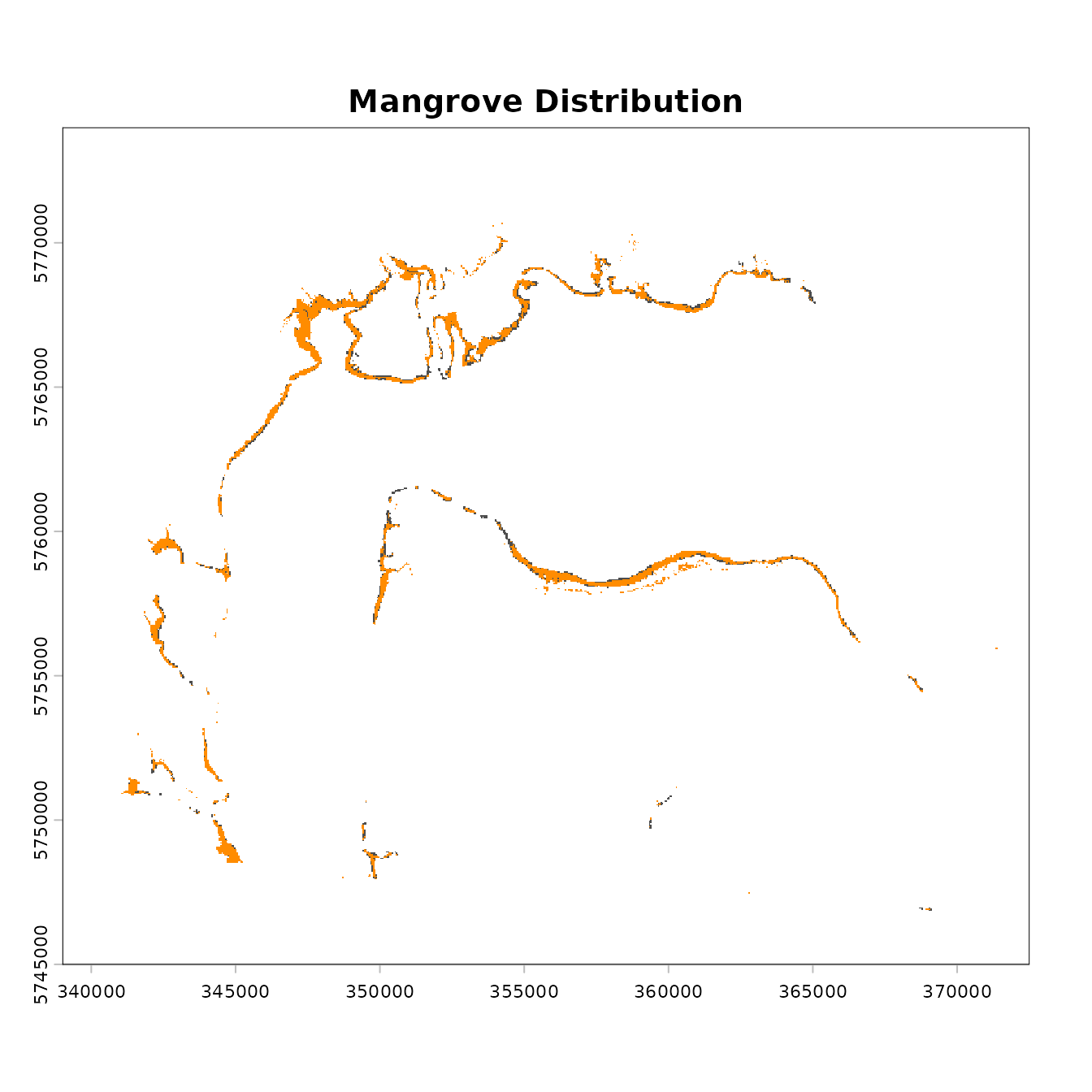
At this stage it is important to check that the data are georectified
(in the right location on Earth). This can be achieved by simply
plotting the map and checking the coordinates. Otherwise, check the
distribution maps against satellite images, perhaps by using packages
such as ggmap, plotgooglemaps,
googleVis etc. It is also important to check that the data
are suitable for the task at hand.
Calculating spatial metrics
We start by calculating the area of the ecosystem. Area is calculated here using the pixel count method, where the number of pixels classified as the ecosystem of interest is multiplied by the area of each pixel, giving the area of the ecosystem distribution. The area calculated is provided in square kilometres.
a.2000 <- getArea(mangrove.2000)
a.2000
## layer value area
## 1 example_distribution_2000 1 13.6557
a.2017 <- getArea(mangrove.2017)
a.2017
## layer value area
## 1 example_distribution_2017 1 12.3336
# you can also calculate areas for both layers at once by combining them into a raster stack:

a <- getArea(c(mangrove.2000, mangrove.2017))
The results: at time 1 (2000), the ecosystem was 13.6557 km2, and at time 2, (2017) the ecosystem was 12.3336 km2.
Rasters with multiple ecosystems or layers
The getArea function is capable of processing rasters
with multiple ecosystems and layers. Layers usually represent time
slices. The function will return a table of areas, with a row for each
ecosystem represented in the raster, and a separate row for each layer
if there are multiple layers.
If you prefer to focus on a single ecosystem or raster value, and you
do not know the value which represents your target ecosystem, you can
plot the ecosystem and use the terra::click function. Once
you know the value which represents your target ecosystem, you can
create a new raster object including only that value, or for smaller
rasters, simply filter your output table to the value(s) of interest.
Here’s an example with a dummy raster.
# Load dummy multilayer raster for example
rstack <- rast(system.file("extdata", "example_raster_stack.tif",
                                    package = "redlistr"))

# If the target ecosystem is represented by value = 5
r.bin <- rstack == 5 # Has values of 1 and 0
# Convert 0s to NAs, if desired.
values(r.bin)[values(r.bin) != 1] <- NA
# get area
getArea(r.bin)
## layer value area
## 1 time1 1 0.001051
## 2 time2 1 0.001139
## 3 time3 1 0.001033
## 4 time4 1 0.001081
## 5 time5 1 0.001192## layer value area
## 1 time1 5 0.001051
## 2 time2 5 0.001139
## 3 time3 5 0.001033
## 4 time4 5 0.001081
## 5 time5 5 0.001192
# note this alternative is slower for large rasters. The getAreaTrend function takes one multilayer raster.
It calculates the area for each layer or list element, for each
ecosystem. The function returns a list of trend class
objects, with one element for each ecosystem or raster value in the
input data.
#input multilayer raster
rstack <- rast(system.file("extdata", "example_raster_stack.tif",
                                    package = "redlistr"))
# returns a list of trends, one per ecosystems
area.trend <- getAreaTrend(rstack)
Now we can summarise the change for ecosystem 1, this function also produces a plot of area over time:
summary(area.trend[[1]])## Summary of ecosystem trend
## ----------------------------
## Net change in area:
## -2.9e-05 kms squared
##
## Modeled change in area:
## -3.292776e-05 kms squared
##
## Modeled percent change in area:
## -4.192725 %
##
## Ecosystem area:
## 0.000762 0.000757 0.000857 0.000735 0.000733
## Input data class: SpatRaster
## Input raster layers: 5
## Raster dimensions: ext(0, 100, 0, 100)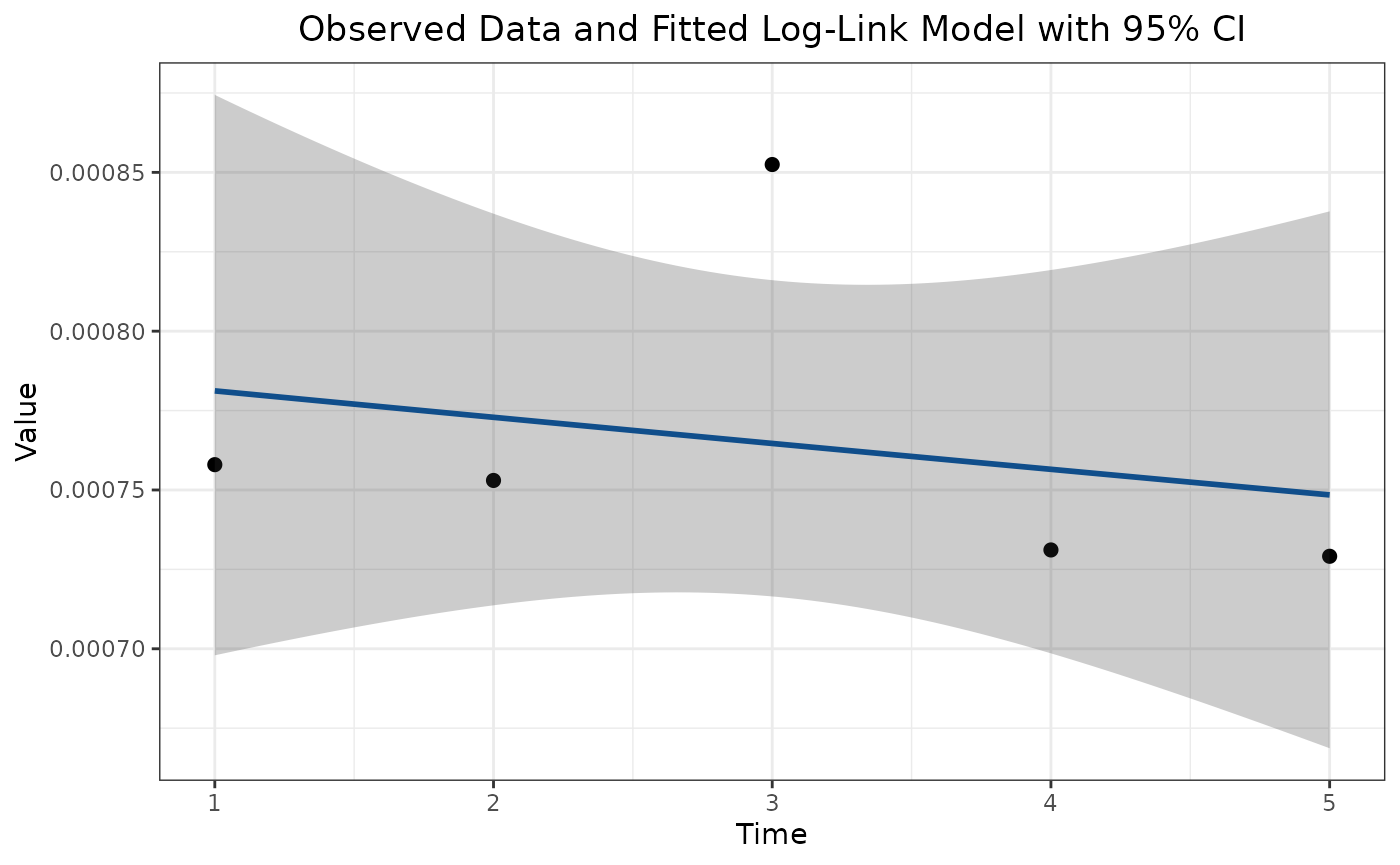
And we can plot the difference between the two ecosystems over the two time points.
plot(area.trend[[1]]@diff)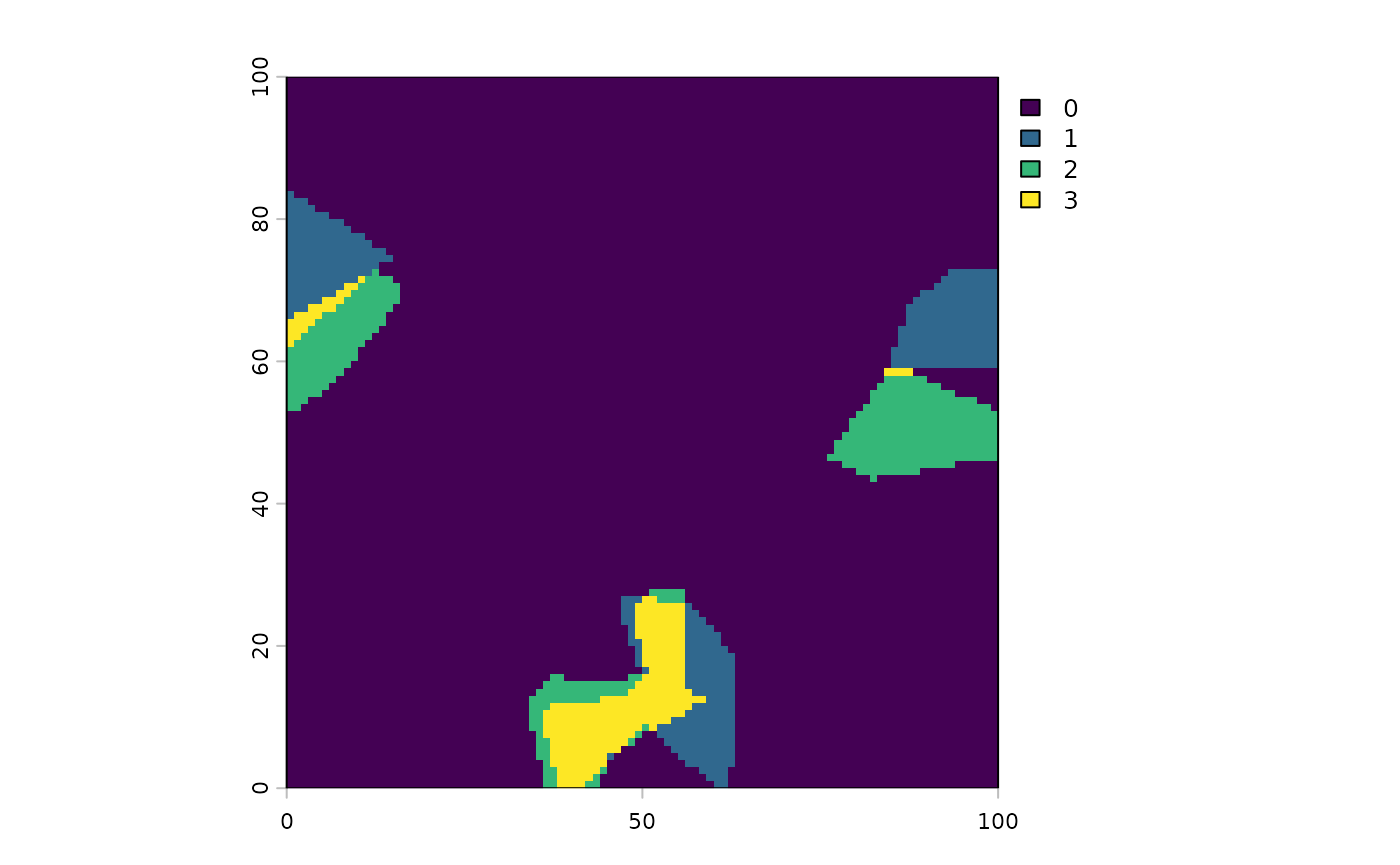
3. Converting from raster to vector format
Functions in this package, like the getEOO and
getAOO functions, work on polygons as well. You can use
functions in packages terra and sf to convert
your data from raster to vector format. For vector format you can
specify which column contains ecosystem names. If all polygons are from
one ecosystem, you can leave out this argument.
mangrove.2000.poly <- as.polygons(mangrove.2000) |> st_as_sf()
#fix crs encoding
st_crs(mangrove.2000.poly)$wkt <- enc2utf8(st_crs(mangrove.2000.poly)$wkt)

EOO.poly <- getEOO(mangrove.2000.poly)
AOO.poly <- getAOO(mangrove.2000.poly)
## Initialising grids## Assembling initial grids## Running jitter on units with 150 or fewer cells## ## jittering n = 354. Working with data in vector format
Importing data as shapefile or .KML file
To import data from a shapefile (.shp) or other common vector
formats, we can use the sf::st_read function.
my.shapefile <- st_read('./path/to/folder/shapefile.shp')
my.KML.file <- st_read('./path/to/folder/kmlfile.kml')
Once these files are imported, they can then be converted into raster
format via the terra::rast or terra::rasterize
functions if desired. However, many of the functions in the package will
accept vector format directly.
Polygon data with multiple ecosystems
If your input data is in polygon format, you can enter the name of the column containing ecosystem labels into the names_from argument. If left empty, for polygon inputs the function will treat all polygons as part of a single ecosystem type.
# polygon example
polygons <- st_read(system.file('extdata/', 'example_polygons.shp',
  package = "redlistr"))
## Reading layer `example_polygons' from data source
## `/home/runner/work/_temp/Library/redlistr/extdata/example_polygons.shp'
## using driver `ESRI Shapefile'
## Simple feature collection with 10 features and 1 field
## Geometry type: MULTIPOLYGON
## Dimension: XY
## Bounding box: xmin: 0 ymin: 0 xmax: 100 ymax: 100
## Projected CRS: WGS 84 / UTM zone 56S
poly_areas <- getArea(polygons, names_from = "time1")The getAreaChange function takes two inputs in the same
format. It calculates the difference in area between two datasets, which
can contain multiple ecosystems. It can accept data from
data.frame such as those output by the
getArea() function, SpatRaster,
SpatVector or sf objects with POLYGON
geometries. Make sure to provide area measure in km2 if you are using a
data.frame as the input. Note that when providing data frame and polygon
inputs, the column name with unique ecosystem labels must be included in
the function call. If the column name is different in the two inputs,
both names must be provided in the same order as the input datasets.
# input rasters
area.change <- getAreaChange(mangrove.2000, mangrove.2017)

# input data frames
# value is the column that identifies the ecosystem in both tables.

area.change <- getAreaChange(a.2000, a.2017, value)

# input polygons
polygonsT5 <- st_read(system.file('extdata/', 'example_polygons_t5.shp',
  package = "redlistr"))
## Reading layer `example_polygons_t5' from data source
## `/home/runner/work/_temp/Library/redlistr/extdata/example_polygons_t5.shp'
## using driver `ESRI Shapefile'
## Simple feature collection with 10 features and 1 field
## Geometry type: MULTIPOLYGON
## Dimension: XY
## Bounding box: xmin: 0 ymin: 0 xmax: 100 ymax: 100
## Projected CRS: WGS 84 / UTM zone 56S
area.change <- getAreaChange(polygons, polygonsT5,
  names_from_x = "time1",
  names_from_y = "time5")